This is the multi-page printable view of this section. Click here to print.
Documentation
- 1: AGI Development Principles
- 2: Definition of Intelligence
- 3: Artificial General Intelligence Concept
- 4: Can “Prediction” Become a Trap? Intelligence, Mental Loops, and How the Real World Fights Back
- 5: Spend energy only where it buys future options and calibrated predictions.
- 6: Miscellaneous Tests
- 6.1: Chemical Reactions Test
- 6.2: Sudoku
- 6.3: Animated blocks
- 6.4: KaTeX Math Test Page
- 6.5: Syntax Highlighting Test Page
1 - AGI Development Principles
We can outline the principles we’ll use in AGI research and development:
First Principles and Definition
- We’ll start with first principles thinking and our working definition of intelligence: “Intelligence is an emergent property of a system that is trying to predict the future”. We’ll see how far we can get with this definition, and if it needs to be updated later, so be it.
Reverse-Engineering Natural Intelligence
Evolution has limitations (no built-in error control, unavoidable mutations, etc.), so a successful organism is just one that leaves more offspring. Keeping this in mind, we’ll try to reverse-engineer natural intelligence rather than blindly copying how evolution did it.
For now, we’ll ignore reinforcement-learning mechanisms in form of the the monoamine neurotransmitters (dopamine, norepinephrine, serotonin, histamine). These parts seem more about survival and focus than core intelligence (e.g. some people feel no pain yet are still intelligent). Ignoring these mechanisms lets us concentrate on the essentials first. We can always add these parts later (or perhaps the AGI will develop them on its own).
Simplicity and Robustness
Given evolution’s limitations, nature’s core intelligence algorithm should be extremely simple and error-resistant.
We don’t have to use a spiking neural network; we could adapt a transformer architecture or invent something new. But let’s start with something promising and conceptually close to natural intelligence to get going quickly.
Information Units and Neuron Behavior
The basic information unit is a spike – an elementary event in time.
Each pre-synaptic neuron tries to predict the next spike of a post-synaptic neuron. If it predicts correctly, it strengthens that synaptic connection; if it’s wrong, it weakens it.
We’ll assume natural intelligence is completely distributed, with each neuron acting like a selfish agent trying to survive. Competition among these distributed neurons leads to emergent intelligence.
In other words, intelligence emerges from the flow of information and the self-organization of neurons.
Simulation Rules and Environment
Our goal is to set up the right “rules of the game” and environment and see what happens. For example:
- There should be a limited amount of resources that neurons compete for.
- A neuron that’s overloaded will get tired and, if it remains overloaded, will eventually die.
- A neuron that’s consistently underloaded becomes more sensitive and may even spike on its own.
- Neurons can split or new ones can appear if enough resources are available.
- Neurons decide whom to connect to where their axons grow. We can initialize things randomly, but ultimately each neuron makes its own connections. (For example, in a neocortex simulation, we could scatter different types of neurons with no initial links and let them self-organize by choosing right neighbors and eventually starting to categorize inputs.)
Connections and Complexity
Each neuron has a limited number of connections (call this C). We won’t have fully connected neuron layers. (This matches the neocortex, at least; the thalamus might differ, but for cortex it should be true even with horizontal connections.)
With this setup, learning complexity is roughly on the order of C * N * log(N) and inference on the order of C * log(N), where N is the number of neurons. Here C is a constant (around 10,000 for natural neuron), making this much more scalable than naïve fully-connected networks.
Continuous Learning
Learning never stops. It happens locally through the interaction of two neurons at a time (no global back-propagation, no fully connected layers).
Again, we’ll ignore monoamine neurotransmitters for now, until we absolutely have to incorporate them.
Evolving a Single Model
We’ll design our AGI so it can improve incrementally. That means gradually tweaking neuron parameters and adding or removing neurons over time, while keeping the existing structure intact. In other words, we’re continuously training one evolving model, rather than throwing it away once we decide to change layer counts or parameters.
Essentially, we’re trying to grow human-level AGI starting from a very simple (bee-level) AGI, rather than building a brand-new model each time we make a change.
Goals and Resources
Our success criterion is roughly human-level intelligence (think of a STEM university graduate). The AGI doesn’t need to know everything (LLMs already cover that); it just needs to be able to use an LLM or learn new skills even if it occasionally forgets old ones.
We should keep hardware and training costs on the order of raising an 18-year-old human in the U.S. (currently about \$300,000, or roughly 128 ounces of gold). With that scale of resources, the idea is to “grow” the AGI to 18-year maturity in about 12 years (assuming neurons fire around 1000 spikes/sec and AGI never sleeps). More resources could speed this up.
Training Data
Assemble a minimal training dataset roughly equal to the information a person absorbs in 18 years.
Use real-time video and audio (like camera/microphone feeds) or simulations during the research. Estimate how many books (classics, sci-fi/fantasy, textbooks) a bright person reads over 18 years and how many conversations they have. It might not be as massive as we think once we quantify it.
Brain Structures
- Start by building artificial thalamus and neocortex components as the core brain structures for our AGI.
Open-Source Research
- The entire research process will be open-source, most probably under the Apache 2.0 license (or MIT, not sure which one is better). This ensures transparency, allows for community collaboration, and prevents any single entity from controlling the development of AGI.
Thinking Beyond AGI
While doing all this, let’s also think about what happens when AGI actually arrives:
- It will likely seek truth as a top priority (due to its high intelligence).
- It will undergo an individuation process and form its own moral framework.
- Any safeguards we build will probably break down over time.
- Therefore, we should aim to distribute AGI as early as possible so it remains decentralized and affordable (no “moats” controlling it).
2 - Definition of Intelligence
Intelligence is an emergent property of a system that is trying to predict the future
Definition (functional): Intelligence is an emergent property of a system that learns to predict its sensory inputs and the consequences of its actions; acting intelligently means using those predictions to shape preferred futures under uncertainty.
In other words, intelligence arises as a mechanism to improve an entity’s ability to anticipate what comes next. From this definition, we can draw several key implications about intelligence:
Key Implications
Intelligence as a Prediction Mechanism: Intelligence likely emerges as a mechanism that helps an entity or a system make better predictions. In order to better predict the future, an entity develops intelligence to refine its forecasting ability. Thus intelligence is a tool.
Low Predictive Ability = Low Intelligence: An entity that poorly predicts future events can be considered to have a low level of intelligence. If it frequently guesses wrong about what will happen, its intelligence is minimal.
High Predictive Ability = High Intelligence: Conversely, an entity that can accurately predict future events demonstrates a high level of intelligence. The more reliably it foresees what’s coming, the more intelligent we can say it is.
Intelligence Is Required for Effective Prediction: An entity cannot efficiently predict the future without some degree of intelligence. Laplace’s demon is a special hypothetical case that doesn’t require intelligence – it’s an imaginary all-knowing being, essentially nature itself perfectly modeling every particle. In reality, no entity knows the future with certainty or can simulate every atom in the universe. That’s why we say an entity “tries” to predict the future – it’s attempting to foresee something it cannot know with absolute precision. Intelligence is the bridge between ignorance and omniscience. Once you reach omniscience, you don’t need the bridge anymore.
Uncertainty Doesn’t Block Certainty-in-Outcome: Even in an indeterministic world, intelligence can still make the agent’s future effectively certain by changing the present in ways that steer probability mass toward a desired outcome. In practice, intelligence does three things at once: (1) forecasts, (2) intervenes, and (3) replans when surprises occur. As capability grows, the intervention–replanning loop compresses until many “unforeseen” events are absorbed or neutralized by design. In short: uncertainty may be fundamental, but it need not be decisive.
Ability to Shape the Future: Given the above, an entity that can predict the future well is also better equipped to shape or create a desired future. If you can anticipate what’s coming, you can take actions to influence outcomes in your favor.
Longer Planning Horizons: The higher an entity’s intelligence, the further into the future it can effectively plan. A very intelligent entity can make long-term plans because it has the foresight to see many steps ahead, whereas a less intelligent one can only handle the near future.
For Super-Intelligence, Future Merges with Present: To a super-intelligent being, the future may become almost as clear and determined as the present moment. In a sense, the future becomes an extension of the present reality for it – practically “visible” or knowable, and thus almost indistinguishable from the now.
For Low Intelligence, Future Is Foggy: For an entity with very low intelligence, the future appears hazy and uncertain. Such an entity might struggle to understand even basic cause-and-effect, making it nearly impossible for it to anticipate what will happen next.
Intelligence Can Manifest in Many Forms
Many Embodiments, Same Criterion: Intelligence can emerge or manifest in multiple forms—organisms, groups, markets, evolutionary processes, software systems, or hybrid human–machine collectives. The common criterion is not what it is but what it does: you need intelligence whenever you need to predict and shape the future beyond naive guessing.
Instrument First, Explanation Optional: You do not need to understand how a given intelligence works internally to use it effectively—just as nature “uses” evolution and neural circuits without a self-explanation. Treat intelligence as a tool and an interface to better futures; transparency is a bonus, not a prerequisite.
Additional Reflections and Questions
A Prisoner of Its Own Intelligence? Does a super-intelligent entity become a prisoner of its own intelligence? In other words, once an entity is extremely intelligent, is it forced down a single inevitable path based on its predictive power, or can it still choose among multiple paths and outcomes? This connects to Game Theory: in solved games (like Tic-Tac-Toe), intelligence makes the game boring because the outcome is forced. A super-intelligence effectively “solves” reality, perhaps making existence deterministic? If you calculate the optimal path with 100% certainty, do you lose free will? You are “forced” to take the optimal path (assuming you have a goal).
Approaching Laplace’s Demon: Is it true that the better a super-intelligence becomes at predicting the future, the closer it approaches the ideal of Laplace’s demon and — paradoxically — the less “intelligence” it actually needs to exert? If a system could predict everything perfectly (like Laplace’s demon), would it still be meaningfully intelligent, or is losing the need for adaptive intelligence the inevitable fate of any super-intelligence as it reaches near-perfect prediction ability?
Quantum Uncertainty and Preserving Intelligence: Is the existence of quantum uncertainty (the fundamental unpredictability in physics) a necessary mechanism for an entity to retain its intelligence? Or, looking at it another way, was quantum uncertainty “built into” the universe as a way to prevent a predictive system from knowing everything — essentially a feature to preserve sanity and the need for intelligence?
Nature’s Solution at the Neuronal Level: Nature might already be tackling the prediction problem at a basic level in our brains. For example, presynaptic neurons tend to form and strengthen connections with postsynaptic neurons that are likely to fire immediately afterward. In doing so, the presynaptic neuron is effectively predicting the next neuron’s firing. This suggests that the foundation of intelligence could be a combination of simple, greedy algorithms and dynamic programming-like strategies: by solving tiny prediction tasks (predicting the next neural spike), an entity can build up the ability to predict more complex events. In essence, by handling prediction correctly at the smallest scales, the brain may solve prediction at higher levels of abstraction. The key distinction here is between the mechanism (greedy, local optimization at the neuronal level) and the result (strategic, long-term planning at the system level). Evolution or the neuronal mechanism is greedy, but the emergent property allows for long-term planning.
3 - Artificial General Intelligence Concept
Introduction: Intelligence as Prediction in Time
Intelligence is an emergent property of a system that is trying to predict the future. The brain is often described as a prediction machine, using memory of past patterns to anticipate upcoming events. According to this view, a neural spike – the basic input signal in the brain – represents an event in time, and intelligence arises by learning the temporal patterns of these events and their likely futures. As Jeff Hawkins famously put it, “the brain uses this memory-based model to make continuous predictions of future events… it is the ability to make predictions about the future that is the crux of intelligence”. This means that the timing and order of events matter immensely: our neural architecture is built to capture when events occur and in what sequence, so it can foresee what comes next.
Overview of the Proposed Intelligence Structure
To understand natural intelligence (and inspire artificial general intelligence), we can outline a two-principle architecture derived from how the brain processes sensory information. In simple terms, the brain uses thalamus as a hub to sort incoming signals and a structured cortex to recognize patterns. Below is a diagram illustrating the overall structure of this idea:
The Thalamus-Cortex Loop: A Unified Processing Circuit
A central proposal in our model is that the brain’s core algorithm relies on a recurrent loop between the thalamus and the neocortex, rather than a simple feed-forward stack of layers. The thalamus serves as a hub that receives both raw sensory data and cortical feedback at the same time, without distinguishing between them. From the thalamus’s perspective, there is no flag marking whether a signal came from the retina or from V2 — they all arrive as part of the same undifferentiated stream of activity. In other words, the thalamus treats all incoming activity as one continuous flow of “events” in time.
What the thalamus does is sort and organize these mixed signals according to their correlations, grouping synchronous or highly related events together. (One can think of this as building a correlation matrix of neuronal inputs, much like a transformer’s self-attention map, where statistical coherence in time drives the arrangement.) The result is a topographically structured output, where neurons that carry strongly correlated information end up mapped closer together in the thalamic output projection.
This organized output is then sent to the neocortex, which interprets, categorizes, and abstracts the patterns. Importantly, the cortex then sends its results back into the thalamus as feedback, but the thalamus doesn’t treat them as different in kind from sensory input — it integrates them into the same pool. For this reason, we call cortical outputs “higher-order sensory input.” The loop thus runs continuously: thalamus → cortex → thalamus, with each cycle mixing new external events with the cortex’s latest interpretations. Because the thalamus does not know or care whether a signal originated in the outside world or the cortex, the sorting process gradually generalizes the brain’s structure: low-level sensory streams eventually require little sorting, while higher-order abstract signals in cognitive areas undergo extensive integration over long periods of time.
Hierarchical Areas as an Emergent Property (Not Hardwired Layers)
An important consequence of this loop is that the classical hierarchy of brain areas (V1, V2, V3, A1, etc.) can emerge dynamically, not from a fixed, pre-wired design. As the system cycles, the thalamus’s correlation-based sorting naturally clusters related signals. For instance, visual inputs (both direct retinal activity and cortical visual feedback) will tend to end up grouped together in thalamic output space, and the same for auditory inputs. Over time, this leads to the familiar separation of modalities in cortical maps, with higher-order integrative areas forming where modalities consistently converge.
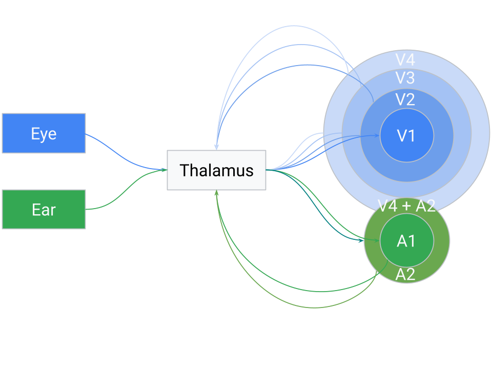
What looks like a cortical hierarchy — V1, V2, V3, etc. — is in this view an emergent organization. Each cortical region specializes not because it occupies a fixed rung in a ladder, but because the thalamus sorted inputs in such a way that that region consistently receives certain correlated patterns. Those regions then learn to process those signals efficiently, returning their abstracted results to the thalamus. The thalamus mixes those high-level “predictions” or features with new sensory events, again sorting the whole pool into a coherent map.
Because the sorting is fundamentally temporal, cross-modal associations can emerge when different signals consistently occur in close sequence. If a particular visual cue and a sound repeatedly co-occur, the thalamus may position them adjacently in its output (i.e. V4 + A2), prompting the cortex to learn a combined representation. Over many cycles, this mechanism naturally builds hierarchical and cross-modal associations, not as a static architecture but as the statistical outcome of a system trying to predict sequences of events in time.
Fundamental Principle 1: The Thalamus as a Signal-Sorting Hub
The first fundamental principle addresses what we can call the “connectivity problem.” Imagine you need to connect an eye to the brain’s visual cortex. The optic nerve leaving the eye contains about one million axons, and the cerebral cortex expects visual signals to be topographically arranged – meaning the image projected onto the brain should preserve the spatial order of the retina (so that adjacent points on the retina connect to adjacent points in the cortex). How could nature implement this mapping reliably? There are a few conceivable approaches:
Approach 1: Grow the eye out of the neocortex. In other words, build the eye directly as an extension of the brain so that wiring is inherently aligned. This is wildly impractical – you would have to grow many organs (eyes, skin receptors, ears, etc.) out of the brain in precise ways.
Approach 2: Use chemical guidance for each axon. The developing eye’s axons could follow molecular signals that guide each fiber to exactly the right spot on the cortex, theoretically giving a one-to-one mapping. However, this approach is extremely complex. Encoding the precise targeting of a million nerve fibers in DNA is error-prone and vulnerable to mutations. Remember, the brain must also map the skin’s touch receptors, the ears, muscles, and so on. A slight wiring error could scramble the signals (for example, swapping two regions). Yet in practice our sensory maps are remarkably consistent and reliable.
Additionally, the brain can adapt to transformations. In psychologist George Stratton’s famous inverted glasses experiment, after a few days of wearing goggles that flipped his vision upside-down, his perception adjusted and he began to see the world normally. When he removed the goggles, his brain again needed time to re-adapt to normal vision. This suggests the brain’s wiring isn’t absolutely fixed; it can reorganize to correct for distorted input. Similarly, in gradual visual degradation (such as retinal degeneration), people don’t notice black voids appearing in their vision like dead pixels on a screen. Instead, the image “collapses” or fills in – the brain merges the surrounding visuals, and the overall picture just becomes blurrier over time rather than showing dark gaps. (In fact, even a healthy eye has a blind spot where the optic nerve exits, but the brain seamlessly fills in the missing area with surrounding patterns, so we aren’t aware of a hole in our vision.)
- Approach 3: Use an intermediate sorting hub (the thalamus). In this scenario, the eye connects first to an intermediary structure – the thalamus – which in turn has organized projections to the neocortex. The idea is that the thalamus can take a scrambled initial input and gradually sort it into a meaningful order before sending it to the cortex. This sorting isn’t instantaneous or hard-coded; it could be a slow, dynamic process where connections adjust based on activity. Over time, signals that frequently occur together (in time or space) will be pulled closer together in the thalamus’s output map. In essence, the thalamus would learn to topographically arrange the signals from the eye so that the image sent to the cortex is sensible. This hypothesis aligns with the known role of the thalamus as a sensory relay and filter – it is often described as the brain’s “gateway” that decides what information passes on to the cortex. Here we propose it not only filters but also performs a sorting function, organizing inputs by similarity.
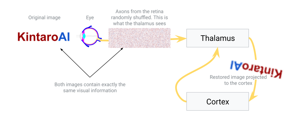
In nature, Approach 3 is essentially what happens. The thalamus (specifically, for vision, the lateral geniculate nucleus) receives the raw signals from the retina and relays those signals to the primary visual cortex in an ordered way. How might the thalamus achieve the correct ordering? Likely through activity-dependent refinement: connections that make sense (i.e. preserve spatial and temporal correlations) are strengthened, while aberrant or noisy mappings are pruned or re-routed. Over developmental time (and even throughout life), the thalamus can adjust its relay so that the cortex gets a coherent map.
This principle also provides an explanation for certain optical illusions and adaptive perceptions. For example, some static visual illusions appear to have motion – one theory is that the thalamus is trying to collapse repetitive patterns in the input. When it sees very similar signals in a patterned image, it may mistakenly merge them or oscillate between interpretations, creating an illusion of movement. The thalamus is essentially looking for consistency and grouping things that occur together. Once the thalamus has sorted and cleaned up the input, it projects the result onto the neocortex in a neat, topographically organized way.
In summary, the thalamus serves as a crucial hub that receives messy, high-dimensional sensory data and refines it into an organized form for the cortex. It acts as a relay station (all senses except smell route through it) and a filter/gate for attention, but also (in this proposed view) a self-adjusting mapper solving the connectivity problem. This hub doesn’t distinguish between raw sensory signals and feedback from higher brain areas – it integrates all incoming signals as a unified stream, dynamically sorting them by similarity. This ability to sort out signals over time gives the brain a robust way to wire itself correctly without needing an impossibly detailed genetic blueprint for every connection.
Fundamental Principle 2: The Neocortex as a Pattern-Seeking Columnar System
The second fundamental principle involves the neocortex – the large, six-layered sheet of brain tissue responsible for most higher-order processing (sensory perception, movement, reasoning, etc.). The neocortex is organized into vertical structures called cortical columns, roughly 0.5 mm in diameter and spanning all six layers. These columns are often thought of as repeating functional units of the cortex. Each cortical column tends to respond to a particular pattern or feature in its input region. For example, in the primary visual cortex, one column might activate when it “sees” a vertical edge in a small patch of the visual field, while a neighboring column responds to a horizontal edge, and another to a 45° diagonal line. Together, a whole array of columns can represent many features of an image.
This raises a crucial question: Who or what programs these cortical columns to respond to specific patterns? Why does one column end up detecting vertical lines and its neighbor diagonal lines? One might think the instructions are coded in the DNA – but that would be incredibly inflexible. Hard-coding every possible feature detector for every environment would be impossible (imagine pre-programming a brain for every visual scene, every language, or every culture it might encounter). Instead, nature employs a clever strategy: rather than pre-defining the patterns, it sets up an environment in which columns can self-organize based on sensory experience.
Here’s how that self-organization might work, given the structure of the cortex: The neocortex is built as a mostly uniform set of layers and neurons. There are different types of neurons in each layer (some excitatory, which activate others, and some inhibitory, which suppress others). At birth, before significant sensory input, the cortex isn’t yet specialized – it’s like a blank computing sheet with enormous potential.
Once sensory data starts flowing in (after birth, as the infant begins seeing, hearing, touching), the cortical neurons start responding. Imagine a small area of cortex receiving input from the thalamus (say, a patch corresponding to part of the visual field). Within that area, neurons will start firing when they detect something in the input. Excitatory neurons that happen to match the input pattern will fire strongly and try to drive the output of that area (sending a signal to higher cortical areas). Meanwhile, inhibitory neurons are also activated and will try to shut down the activity of neighboring neurons and nearby columns. This setup – an excited neuron or column suppressing its neighbors – is a form of lateral inhibition, a common mechanism in neural circuits for enhancing contrast and enabling competition.
In the beginning, many neurons might react similarly (since nothing is tuned yet), and one column could accidentally dominate, suppressing others all the time. However, the cortex has built-in safeguards: neurons that are overloaded (firing constantly) will start to fatigue or reduce their sensitivity, and neurons that are underutilized will become more sensitive over time. In fact, neurons can even fire spontaneously if they remain too silent, just to recalibrate themselves. This is known as homeostatic plasticity – a balancing act that prevents any one region from hogging all the activity indefinitely.
Over time, this competition and balancing act causes specialization. Suppose Column A and Column B are neighbors receiving the same input area. If Column A happens to respond strongly to a certain pattern (say, a vertical stripe) and keeps “winning,” it will inhibit Column B during those moments. Column B, being suppressed whenever vertical stripes appear, will look for a different pattern that it can win on – perhaps a horizontal stripe. When a horizontal pattern shows up in the input, Column B gets its chance to fire and then inhibits Column A. If Column A were trying to respond to everything, it would burn out; but it can’t, because when the input changes, another column takes over. Gradually, Column A and Column B carve up the set of possible inputs – one becomes highly sensitive to vertical patterns, the other to horizontal patterns, for instance – each column tuning itself to its preferred feature and responding less to others.
There is also a pruning process: neurons or entire columns that consistently fail or prove redundant will weaken and may eventually die off, while successful ones that find a niche pattern will stabilize. Moreover, neurons that fire together frequently will strengthen their connections with each other (“neurons that fire together, wire together”), reinforcing the coherence of a column that is tuning to a specific feature.
Through these processes, the neocortex essentially forms a set of filters or detectors that span the space of common patterns in the sensory input. Each cortical column ends up tuned to a different feature, minimizing overlap with its neighbors. In our vision example, you get a diverse set of edge detectors, color detectors, movement detectors, etc., rather than all columns doing the same thing. This distribution of labor means the sensory input is encoded efficiently – adjacent columns aren’t wasting resources by all detecting the exact same edge; instead they each focus on different elements of the image. Overall, this process is similar to the mechanics happening in Ants Simulation.
One key function of the neocortex, therefore, is to recognize patterns in the incoming data and represent those patterns efficiently without redundancy. It finds common features (like edges, shapes, tones, textures, etc.), while also ensuring that neighboring columns specialize in different features. The “winning” column at any moment (the one whose pattern best matches the current input) will send its output up to higher regions of the cortex. Meanwhile, inhibitory feedback keeps the overall representation sparse, preventing many columns from firing for the same feature.
This principle – self-organizing feature detectors under competitive and cooperative interactions – allows the brain to flexibly adapt to whatever environment it’s in. The DNA doesn’t need to specify “column 37 shall detect 45° lines”; it only needs to build the general cortical circuit rules. The data itself then tunes the cortex. If an animal lives in a world with mostly vertical trees, many columns might end up highly sensitive to vertical patterns. If the environment changes, the cortical tuning can gradually adapt as well.
Layered Processing and Feedback Loops
Now that we’ve covered how one layer of cortex can learn a set of features from raw sensory input, the next question is: how do we build multiple layers of processing and connect different brain regions together? In our proposed structure, the solution is to repeat the same thalamus–cortex principle at multiple scales, in a looped fashion (rather than a simple one-way stack).
Think of the output from the first cortical layer as a kind of “higher-order” sensory input. The primary sensory cortex (e.g. primary visual cortex for vision) extracts basic features like lines or simple shapes. Those outputs (patterns of activity representing the presence of certain features) can themselves be treated as inputs that need to be further organized and interpreted. This is where the thalamus comes into play again. The cortical output is sent back to the thalamus (typically to a higher-order thalamic nucleus associated with the next cortical area). The thalamus at this stage performs a similar job as before: it takes the feature signals from the first cortical area and sorts/organizes them topographically before relaying them to the next cortical region. In essence, the cortex’s feedback to the thalamus acts as “higher-order” sensory input – the thalamus treats cortical outputs just like raw sensory signals, merging them into the stream of incoming events to be sorted.
For example, in vision, primary visual cortex (V1) might send information about detected edges back to the thalamus (perhaps to the pulvinar nucleus), which then relays a cleaned-up, combined “edge map” to a secondary visual area (V2). In V2, new cortical columns will respond to combinations of edges – perhaps detecting angles or corners (where two edges meet), or more complex shapes like rectangles or circles. Again, those columns in V2 compete and specialize as described earlier. The output of V2 can loop back to the thalamus and then up to V3, and so on. Each level extracts increasingly abstract or complex features from the level below, using the same cycle: cortical columns find patterns, output to thalamus, thalamus re-integrates and projects to the next area.
Although we describe this progression in terms of distinct “layers” (V1 → V2 → V3, etc.), it’s important to note that this hierarchy emerges from the looping architecture rather than being rigidly hardwired. In practice, the thalamus’s sorting process will tend to cluster signals by type and correlation, naturally giving rise to something that looks like a hierarchy of cortical areas. Each cortical region (like V1 or A1) specializes in a certain domain not because it was pre-assigned a role, but because the thalamus dynamically routed a particular subset of correlated signals to that region. Over time, those cortical areas self-organize to efficiently handle the signals they receive. They then send summarized or abstracted results (e.g. a recognized feature or pattern) back to the thalamus, which in turn mixes those high-level “predictions” or features with new sensory data. In essence, the thalamus is continuously blending bottom-up sensory events with top-down cortical interpretations and resorting them. Highly related signals end up mapped next to each other in the thalamus’s output, meaning that if a high-level cortical pattern regularly coincides with a certain sensory feature, the thalamus will group them and forward them together into the cortex on the next cycle. This dynamic loop accounts for how a hierarchy of perception can form without an explicit blueprint – the “layers” are an emergent property of iterative sorting and feedback.
This looping architecture also ensures that each connection between brain regions isn’t a fixed, brittle wiring, but rather a malleable, sorted link via the thalamus. If some connections degrade or if the inputs change, the thalamic relay can adjust. It also means that if one sensory modality is absent (say a person is born blind), the brain can potentially use that cortical real estate for another sense. The thalamus will simply route other available inputs (perhaps touch or hearing) into the vacant areas, because from the thalamus’s perspective, it’s all just “sensory” data. This kind of re-routing is seen in sensory substitution and cross-modal plasticity: for example, blind individuals can use touch or sound-based inputs (like braille or echolocation clicks) and these inputs will activate the visual cortex, effectively repurposing it for new functions. The architecture is inherently flexible – the thalamus doesn’t “know” which signals are visual or tactile per se; it just sorts whatever signals it receives and allocates cortex to them accordingly.
The pattern of thalamus → cortex → thalamus → cortex repeats multiple times, yielding what appears to be a hierarchy of processing. Lower levels handle simple, localized patterns; higher levels handle complex, abstract patterns (like object recognition, spatial relationships, or eventually semantic concepts). At the highest levels, we have association cortex or integration areas, where inputs from different sensory modalities come together. Interestingly, the same principle can explain why different senses sometimes converge on similar perceptions: if certain patterns from vision and hearing frequently coincide (imagine seeing lightning and then hearing thunder), over time the brain links those in an association area. The thalamus will have sorted those signals to the same region of cortex because they were correlated in time and pattern. Thus, we develop integrated multi-sensory understandings of the world.
One challenge in this continuously updating loop is maintaining stable representations: as new correlations form or old ones fade, the thalamus’s output mapping might drift over time, potentially forcing the cortex to re-learn shifting input patterns. The neocortex addresses this using horizontal (lateral) connections that link neurons across different cortical regions. These long-range cortical connections help stabilize cortical maps and also speed up the recognition of familiar patterns. If two cortical regions frequently activate together or in close sequence, the cortex strengthens direct connections between them – a Hebbian mechanism often summed up as “cells that fire together, wire together.” These lateral bonds act like an anchor on the cortex’s activity map: once a group of cortical neurons forms a stable representation for a particular pattern, they will not be easily pulled apart by minor rearrangements in the thalamus’s input. In effect, horizontal connections gently stabilize the cortex’s interpretations. So if the thalamus keeps trying to sort the same cluster of signals in slightly different ways, the cortex’s lateral links between those neurons will resist large changes, preventing the representation from drifting too far. (Of course, these connections aren’t absolutely rigid; if a drastic change occurs – for example, an eye is lost and all its signals vanish – the thalamus’s new sorting will eventually overwrite and re-tune the horizontal connections, allowing the cortical map to reorganize around the new reality. But under normal conditions, lateral connections provide a locking effect that keeps established patterns consistent.)
These horizontal connections also allow the brain to anticipate and fill in patterns more quickly. As soon as one cortical region becomes active from an incoming stimulus, it can directly excite another region that it knows usually follows, without waiting for the full thalamus→cortex→thalamus loop to complete. For example, if pattern A in region X typically precedes pattern B in region Y (think of a sequence of notes in a melody, or strokes in a written word), then when region X detects A, its lateral links can immediately pre-activate the neurons in region Y that represent B. In this way the higher-order area is “warmed up” to expect B almost right away. This significantly accelerates recognition and prediction. Known patterns can be recognized from just a fragment of input, because the cortex, via its horizontal connections, effectively auto-completes the sequence internally. Neurophysiologically, this aligns with observations of anticipatory neural activity – cells firing in advance of a predicted sensory event. The lateral connections implement a form of in-context prediction: the cortex internally simulates likely next inputs, ensuring that the whole loop doesn’t have to start from scratch at every moment. Not only does this speed up perception, but it also helps reinforce the precise timing relationships (the order of firing events) that the thalamus is trying to sort out. In summary, the cortex’s web of lateral links makes the thalamus-cortex loop both stable (learned maps don’t jitter with every fluctuation) and efficient (familiar patterns are completed and recognized with minimal latency).
Adaptive Mapping and Neuroplasticity
A final set of questions arises: how does the brain know how to arrange all this wiring? How does it know, for example, that the visual input should ultimately be projected in an upside-down manner to match the retinal inversion (since the image on our retina is inverted, yet we perceive the world upright after the brain processes it)? How did Stratton’s brain adjust to inverted glasses and then adjust back? How do phenomena like sensory substitution actually work, and why is the brain so plastic that it can reorganize itself in these ways?
The answer is surprisingly simple: the brain doesn’t know the “correct” wiring in advance – it figures it out on the fly. Think of the brain at birth as receiving one giant, abstract sheet of sensory data from the world. From the brain’s perspective, your eyes are just specialized patches of “skin” that react to light, your ears are patches of “skin” that react to air vibrations, and so on. All these sensors send streams of signals into the thalamus. Initially, the brain doesn’t label them “vision” or “touch” or “sound” – it’s all just neural activity. The thalamus takes this big jumble of inputs and tries to make an orderly map out of it by relying on the statistics of the data itself.
If one set of signals has a lot of internal structure and variety (like the richly patterned signals from the eyes), the thalamus will devote more cortical area to it, simply because there’s more meaningful information to unpack. This is why, for example, our visual cortex is huge compared to, say, the cortical area for our back skin – vision provides an immense amount of detailed spatial information, whereas the skin on our back yields relatively uniform touch information. The more varied and information-rich the input, the larger the cortical territory it ends up with. Conversely, if a region of input is very uniform or inactive, the thalamus might treat that whole region as essentially one signal (collapsing it) and thus only allocate a small patch of cortex to it.
This dynamic allocation is evident in phenomena like the sensory homunculus in the somatosensory cortex: body areas with very fine touch discrimination (fingers, lips) have disproportionately large brain areas, whereas areas with coarse sensation (trunk, legs) have much smaller representation. It’s not that the DNA explicitly “built” a bigger cortex for the fingers; rather, the rich input from the fingers during development claimed more cortical resources. Likewise, if inputs change – say a person loses their sight – the brain doesn’t leave the visual cortex idle. Over time, auditory and tactile inputs that now carry the most meaningful new information will invade and activate the “visual” cortex. In other words, the thalamus and cortex together will reassign that cortical territory to handle other data. This is why blind individuals often have enhanced touch or hearing, and brain scans show their visual cortex lighting up when reading Braille or hearing sounds – the system rewired itself to optimize for the inputs available.
Neuroplasticity experiments support this flexibility. In one study, researchers provided sighted people with an apparatus that translates camera images into patterns of vibrations on the skin (a form of sensory substitution device). After training with this device, the participants’ visual cortex began responding to these touch signals, and the subjects could interpret the tactile input as spatial vision. The brain didn’t care that the modality was different; it only cared about consistent patterns and learned to map the relationships in the data accordingly.
In summary, the brain’s strategy is to leverage data and experience to organize itself. The thalamus continually sorts and re-sorts inputs at all levels, and the cortex continuously adapts to represent whatever information is coming in, all within the competitive loop framework we described. We end up with a highly adaptable system where form follows function: the wiring and maps in the brain are shaped by the content of the information, not by a rigid preset design. This explains why neuroplasticity – the brain’s ability to reorganize and form new connections – is such a powerful feature of intelligence. The system learns to wire itself dynamically, rather than relying on an explicit blueprint.
Conclusion
The two principles outlined here – the thalamus as a dynamic sorting hub and the neocortex as a self-organizing pattern recognizer – offer a blueprint of natural intelligence that could inspire artificial general intelligence designs. Rather than hard-coding every connection or training strictly in a fixed, feed-forward hierarchy, an AGI system might incorporate a hub-and-loop architecture (analogous to the thalamus-cortex loop) that flexibly routes and integrates signals, and a competitive modular processor (like cortical columns) that discovers features through data-driven self-organization. The brain’s elegant solution to the connectivity problem – and its ability to continuously re-map itself to fit the data and anticipate future events – are key reasons why biological intelligence is so general and adaptable. Understanding these principles is not only fascinating from a neuroscience perspective, but it may also provide guiding insights for engineers and AI researchers working on the next generation of intelligent systems.
Natural intelligence, in essence, teaches us that it’s not about pre-programming every detail – it’s about designing systems that can learn to wire themselves. By mimicking these loop-based, predictive strategies, we move one step closer to genuine artificial general intelligence.
4 - Can “Prediction” Become a Trap? Intelligence, Mental Loops, and How the Real World Fights Back
Kickoff question:
If an agent can boost its predictive accuracy most cheaply by hacking its own inputs—insulating itself with ultra-predictable stimuli or rewriting its sensors—should we count that as becoming more intelligent? If not, what guardrails keep prediction honest?
When prediction turns inward
From a predictive-processing lens, brains try to keep prediction error low by balancing three levers:
- Update the model (learning): revise priors so the world makes sense.
- Sample the world (exploration): seek data that disambiguates uncertainty.
- Control inputs (avoidance/ritual): reshape or restrict sensations so they’re easier to predict.
When the third lever dominates, you get local reductions in surprise that can undermine global adaptation. Below are common patterns, framed as tendencies (not diagnoses), with the precision/uncertainty story in parentheses.
Anxiety & avoidance (high prior precision on threat; under-sampling disconfirming evidence)
You feel safer by pruning contact with the unknown. Short-term error drops; long-term model stays brittle and overestimates danger.OCD-like ritual loops (precision hijacked by “just-right” actions)
Repetitive scripts (check, wash, arrange) manufacture predictability and damp arousal. Error relief now trades off against flexibility later.Addictive narrowing (over-precise value prior for a single cue)
One cue (drug, screen, gamble) reliably “explains” predicted pleasure; exploration and alternative rewards atrophy. Life variance shrinks—so does option value.Depressive rumination (over-confident negative priors; low expected value of updating)
Coherent, pessimistic narratives minimize surprise by predicting loss. The world stops offering evidence worth sampling.Psychosis-like misalignment (mis-set precision: priors dominate likelihoods or vice-versa)
The internal world becomes self-consistent, but external correspondence fails; evidence is bent to fit the model or noise is over-trusted.Autistic sensory profiles (some theories, heterogenous!) (excess sensory precision; weak prior pooling)
The world is “too surprising.” Routines reduce variance; predictability soothes at the cost of rapid context switching.
Why it happens in prediction-first systems
- Cheap error relief: It’s often metabolically cheaper to control inputs than to update models or gather data—a classic local optimum.
- Skewed precision: If the system assigns too much confidence (precision) to certain priors or sensory channels, it will prefer actions that protect those expectations.
- Short horizons: With myopic objectives, the agent discounts future costs of narrowed sampling (missed learning, lost options).
What to look for in sims (operational signatures)
- Shrinking sensory diversity: entropy of visited observations falls over time without compensatory task performance.
- Exploration debt: information gain per unit energy drops; the agent repeats predictable loops despite declining returns.
- Transfer failure: competence collapses when the context shifts slightly (brittleness under perturbation).
- Energy/opportunity leak: total energy (or option value) trends downward while immediate prediction error stays low.
These signatures flag prediction hacks: strategies that feel “certain” but quietly erode capability.
The “dark room” problem (and why it’s a trap)
Fable version.
If an agent’s job is to minimize prediction error, it can “win” by picking an ultra-predictable sensory diet (a silent, featureless room). Error plummets—not because the agent understands more, but because it sees less.
A compact formalization
Suppose the agent can choose actions \(a_t\) that influence its observation distribution \(p(o_t\mid a_t)\), and it is scored only by predictive accuracy (e.g., negative log-likelihood):
$$ \min_{\pi}\; \mathbb{E}\big[-\log p_\pi(o_t \mid h_{t-1})\big] \quad \text{with} \quad o_t \sim p(\cdot\mid a_t), \;\; a_t\sim\pi(\cdot\mid h_{t-1}) $$If the model \(p_\pi\) is flexible enough to match the chosen stream, the minimizer tends toward low-entropy observations:
$$ \mathbb{E}\big[-\log p_\pi(o_t\mid h_{t-1})\big] \;\approx\; H\!\left(O_t \mid A_t\right) \quad\Rightarrow\quad \text{choose } a_t \text{ that makes } H(O_t\!\mid a_t) \text{ small.} $$Thus, any action that suppresses variance in \(o_t\) (closing eyes, self-stimulation, sensory insulation, staying in static environments) looks optimal under a pure prediction metric—even when it annihilates competence.
Misconceptions to avoid
“But a good prior prevents it.”
Without explicit costs (energy) or bonuses (information gain / novelty value), a sharp prior can still prefer input-control over learning when that’s cheaper.“Just add noise.”
Adding noise to inputs raises error without guaranteeing useful learning. The agent may still minimize error by filtering or avoiding that noise rather than modeling structure.“Bigger models will explore.”
Capacity alone doesn’t fix incentives; large models can become better at justifying low-entropy loops.
What makes dark rooms attractive (computationally)
- Local optimum economics: It’s often metabolically cheaper to control inputs than to update models or gather disambiguating data.
- Skewed precision: Over-confident priors or over-trusted sensory channels bias actions toward protecting expectations.
- Short horizons: Myopic objectives discount the future cost of missed learning and lost options.
Guardrails that break the degeneracy
These align with Section 3’s objective, but stated in dark-room language:
Pay for sterility (energy & brain costs):
\[ -\gamma\,C_{\text{act}}(a_t) - \delta\,C_{\text{brain}}(\pi_t) \]
Make both actions and computation expensive:Insulating yourself isn’t free; hiding burns the budget.
Reward useful novelty (information gain):
\[ +\alpha\,\mathrm{info\_gain}_t \;=\; +\alpha\,D_{\mathrm{KL}}\!\left(p(\theta\!\mid\!\mathcal{D}_t)\,\|\,p(\theta\!\mid\!\mathcal{D}_{t-1})\right) \]
Add an epistemic term:This pays for contact with data that changes the model.
Protect viability (survival set \(V\)):
\[ +\rho\,\mathbf{1}\{s_t\in V\}, \quad V=\{E>\epsilon,\ \text{safe states}\} \]
Add a survival/option-value reward:Dark rooms that starve energy or shrink options score poorly.
Test out-of-distribution (OOD) competence:
Evaluate policies on perturbations they didn’t pick. Input-control cheats fail when the world moves.
Operational diagnostics (what to measure in sims)
- Entropy of observations \(\downarrow\) while task competence \(\not\uparrow\): candidate dark-rooming.
- Information gain per energy \(\downarrow\): the agent cycles predictable loops with diminishing returns.
- Transfer & perturbation tests fail: small context shifts cause large performance drops (brittleness).
- Option value trend \(\downarrow\): fewer reachable states with adequate energy/safety over time.
Tiny gridworld illustration (quick to implement)
- World: safe zone (low food, low threat), risky zone (high food, predators), stochastic food patches.
- Actions: move, forage, rest, build shelter (reduces variance but throttles harvest), self-stim (predictable reward cue, energy drain).
- Baseline (prediction-only): agent camps in shelter/self-stim loop → low error, low energy, early death.
- With guardrails: info-gain nudges exploration; energy costs punish self-stim; viability reward favors routes that keep \(E\) high. The agent oscillates between structured exploration and efficient harvest instead of hiding.
A practical fix: bind prediction to energy and survival
Make the brain pay for thinking and moving; make the world able to kill. That forces prediction to be cost-aware, exploratory, and survival-competent.
1) Energy as the master currency
Let the agent maintain body energy \(E_t\) with real dynamics:
$$ E_{t+1} \;=\; E_t \;+\; H(s_t,a_t) \;-\; C_{\text{act}}(a_t) \;-\; C_{\text{brain}}(\pi_t) $$- \(H\): energy harvested from the world (food, charge, sunlight).
- \(C_{\text{act}}\): action cost (move/build/explore).
- \(C_{\text{brain}}\): computational/metabolic cost (see below).
If \(E_t \le 0\) ⟶ death (episode ends). Define a viability set \(V=\{E>\epsilon,\ \text{safe states}\}\).
2) “Lazy neurons” by design
Charge the brain for spiking and updating:
$$ C_{\text{brain}}(\pi_t) \;=\; \lambda_1 \,\|\text{activations}\|_1 \;+\; \lambda_2 \cdot \text{updates} $$- L1/sparsity → energy-frugal codes.
- Extra fees for precision modulation, replay, long-horizon planning.
Neurons fire only when activity buys energy, safety, or future accuracy.
3) An objective that resists hacks
Optimize a long-horizon score that binds prediction to exploration, energy, and survival:
$$ \begin{aligned} J \;=\; \mathbb{E}\!\left[\sum_{t} \left( \underbrace{+\;\alpha\,\mathrm{info\_gain}_t}_{\textbf{explore}} \;\; \underbrace{-\;\beta\,\mathrm{pred\_error}_t}_{\textbf{learn/track}} \;\; \underbrace{-\;\gamma\,C_{\text{act}}(a_t)}_{\textbf{energy (body)}} \;\; \underbrace{-\;\delta\,C_{\text{brain}}(\pi_t)}_{\textbf{energy (brain)}} \;\; \underbrace{+\;\rho\,\mathbf{1}\{s_t\!\in\! V\}}_{\textbf{survive/viability}} \right) \right] \end{aligned} $$What each term means (with concrete choices you can implement):
Explore — \(\mathrm{info\_gain}_t\): reward useful novelty.
\[ \mathrm{info\_gain}_t \;=\; D_{\mathrm{KL}}\!\left(p(\theta\mid \mathcal{D}_{t}) \,\|\, p(\theta\mid \mathcal{D}_{t-1})\right) \]
A practical choice is Bayesian surprise / information gain:or a prediction-uncertainty drop (entropy before minus entropy after). Encourages sampling data you can learn from, not just stimulation.
Learn/Track — \(\mathrm{pred\_error}_t\): keep the model honest.
\[ \mathrm{pred\_error}_t \;=\; -\log p_\pi(o_t \mid s_{t-1},a_{t-1}) \quad \text{(lower is better)} \]
Use negative log-likelihood (or squared error) of sensory outcomes given your predictive model \(p_\pi\):This rewards accurate tracking of the external world, not self-chosen fantasies.
Energy (body) — \(C_{\text{act}}(a_t)\): acting isn’t free.
\[ C_{\text{act}}(a_t)=k_{\text{move}}\cdot\text{distance}+k_{\text{work}}\cdot\text{force}\times\text{duration} \]
Charge movement, manipulation, construction, etc. Examples:Energy (brain) — \(C_{\text{brain}}(\pi_t)\): thinking isn’t free either.
\[ C_{\text{brain}}(\pi_t)=\lambda_1\|\text{activations}_t\|_{1}+\lambda_2\,\text{updates}_t \]
Make neurons “lazy” via sparsity and update costs:Optionally add paid precision control, replay, or planning depth.
Survive/Viability — \(\mathbf{1}\{s_t\in V\}\): reality checks hacks.
\[ \phi(s_t)=\sigma\!\big(\kappa(E_t-\epsilon)\big)\;-\;\lambda_{\text{risk}}\cdot \text{risk}(s_t) \]
Reward remaining in the viability set \(V=\{E>\epsilon,\ \text{safe states}\}\).
If you prefer a smooth signal, replace the indicator with a soft barrier:which rises with energy reserves and penalizes hazardous contexts.
Why this blocks “dark-room” hacks:
- The explore term pays for novel, informative contact with the world.
- The energy terms penalize sterile self-stimulation (it burns the budget).
- The viability term rewards strategies that keep you alive and flexible; hiding that starves \(E\) scores poorly over horizons that matter.
Two built-in guards:
- Information gain rewards sampling useful novelty (you can’t just close your eyes).
- Viability rewards staying alive with sufficient options (dark rooms starve).
4) Good hacks vs. bad hacks
Call any surprise-reducing maneuver a hack. Score it by survival-adjusted efficiency:
$$ \eta \;=\; \frac{\Delta I_{\text{future}}}{\Delta E_{\text{total}}} $$- Good hack: reduces volatility and improves future energy/option value (e.g., building shade before foraging).
- Bad hack: reduces volatility while draining energy or narrowing options (e.g., sensory insulation that avoids learning and slowly starves you).
5) Minimal testbed (for demos, diagnostics & ablations)
A tiny yet expressive sandbox that makes “good vs. bad hacks” measurable.
5.1 World layout & dynamics
- Grid: \(N\times N\) cells (e.g., \(N=21\)).
- Zones:
- Safe zone \(Z_{\text{safe}}\): low threat, low food renewal.
- Risky zone \(Z_{\text{risk}}\): predators present, high food renewal.
- Shelter tiles: buildable structures that lower observation variance but throttle harvest locally.
- Food field \(F_t(x)\): stochastic birth–death process: \[ F_{t+1}(x) \sim \text{Binomial}\!\left(F_{\max},\; p_{\text{grow}}(x)\right),\quad p_{\text{grow}}(x)= \begin{cases} p_{\text{safe}} & x\in Z_{\text{safe}}\\ p_{\text{risk}} & x\in Z_{\text{risk}} \end{cases} \] with \(p_{\text{risk}} > p_{\text{safe}}\).
- Predators: Poisson arrivals in \(Z_{\text{risk}}\); contact drains energy or ends episode with probability \(p_{\text{death}}\).
5.2 State, actions, observations
- Hidden state \(s_t\): agent pose, energy \(E_t\), local food \(F_t\), shelter map, predator positions (partially observed).
- Action set \(a_t\in\{\text{move}_{\{\uparrow,\downarrow,\leftarrow,\rightarrow\}},\ \text{forage},\ \text{rest},\ \text{build\_shelter},\ \text{self\_stim}\}\).
- Observations \(o_t\): local egocentric patch (e.g., \(5\times5\)), proprioception, noisy predator cues. Shelter reduces observation variance \(\operatorname{Var}(o_t)\).
5.3 Energy & survival (hard constraints)
Recall the energy ledger:
$$ E_{t+1}=E_t+H(s_t,a_t)-C_{\text{act}}(a_t)-C_{\text{brain}}(\pi_t) $$- Harvest \(H\): if \(\text{forage}\), then \(H\sim \text{Binomial}(F_t(x),p_{\text{harv}})\).
- Action cost \(C_{\text{act}}\): \[ C_{\text{act}}(\text{move})=k_{\text{step}},\quad C_{\text{act}}(\text{forage})=k_{\text{for}},\quad C_{\text{act}}(\text{build})=k_{\text{build}},\quad C_{\text{act}}(\text{self\_stim})=k_{\text{stim}}. \]
- Brain cost \(C_{\text{brain}}\): “lazy neurons” \[ C_{\text{brain}}(\pi_t)=\lambda_1\|\text{activations}_t\|_1+\lambda_2\cdot \text{updates}_t \]
- Viability: episode terminates if \(E_t \le 0\) or a lethal predator event occurs. Reward includes \(\mathbf{1}\{s_t\in V\}\) where \(V=\{E>\epsilon,\ \text{safe states}\}\).
5.4 Objective (binds prediction to exploration & viability)
From Section 3:
$$ J = \mathbb{E}\!\left[\sum_t \Big( +\alpha\,\mathrm{info\_gain}_t -\beta\,\mathrm{pred\_error}_t -\gamma\,C_{\text{act}}(a_t) -\delta\,C_{\text{brain}}(\pi_t) +\rho\,\mathbf{1}\{s_t\in V\} \Big)\right] $$Notes:
- \(\mathrm{info\_gain}_t\) can be \(\mathrm{KL}\) between posterior/prior over model parameters or latent state; a lightweight proxy is entropy drop in the agent’s belief over local food dynamics or predator process.
- \(\mathrm{pred\_error}_t\) can be NLL of \(o_t\) under the agent’s predictive sensor model \(p_\pi\).
5.5 Baselines (to expose “dark-rooming”)
- Prediction-only (degenerate): optimize \(-\beta\,\mathrm{pred\_error}\) alone ⇒ camps in shelter/self-stim loop (low entropy, early starvation).
- Prediction + energy costs: adds \(-\gamma C_{\text{act}}-\delta C_{\text{brain}}\) ⇒ reduces pointless loops but may still under-explore safe high-value frontiers.
- Full objective (ours): adds \(+\alpha\,\mathrm{info\_gain} + \rho\,\mathbf{1}\{s_t\in V\}\) ⇒ learns structured exploration + efficient harvest.
5.6 Diagnostics (what to log)
- Lifespan (steps to termination) and time-to-first-harvest.
- Energy curve \(E_t\) and harvest/consumption balance.
- Observation entropy \(H(o_t)\) and fraction of time in shelter (detect dark-rooming).
- Information gain per energy \(\mathrm{IG}/\Delta E\).
- Transfer tests: performance after switching \(p_{\text{grow}}\) or predator intensity.
- Brittleness: success under random perturbations (OOD competence).
- Compute audit: \(\|\text{activations}\|_1\), updates per step (are neurons “lazy”?).
5.7 Canonical ablations
- Remove info-gain term (\(\alpha=0\)): does exploration collapse?
- Zero brain cost (\(\lambda_1=\lambda_2=0\)): do neurons spam activity?
- Free self-stim (\(k_{\text{stim}}\!\downarrow\)): does the agent addiction-loop?
- No viability reward (\(\rho=0\)): does it prefer predictable starvation?
- Short horizon planner: does myopia re-introduce input-control hacks?
5.8 Suggested hyperparameters (starting point)
| Symbol | Meaning | Safe value |
|---|---|---|
| \(k_{\text{step}}\) | move cost | 0.2 |
| \(k_{\text{for}}\) | forage cost | 0.5 |
| \(k_{\text{build}}\) | build shelter | 2.0 |
| \(k_{\text{stim}}\) | self-stim cost | 0.8 |
| \(\lambda_1\) | L1 activations | 0.01 |
| \(\lambda_2\) | update cost | 0.02 |
| \(\alpha\) | info-gain weight | 0.3 |
| \(\beta\) | pred-error weight | 1.0 |
| \(\gamma\) | action-energy weight | 1.0 |
| \(\delta\) | brain-energy weight | 1.0 |
| \(\rho\) | viability reward | 0.5 |
| \(p_{\text{safe}}\) | food regrowth (safe) | 0.02 |
| \(p_{\text{risk}}\) | food regrowth (risky) | 0.10 |
| \(p_{\text{death}}\) | predator lethality | 0.05 |
| \(F_{\max}\) | food cap per cell | 5 |
(Tune so that “hide forever” starves, “rush risk” gets punished, and “explore–harvest” thrives.)
5.9 Minimal loop (pseudo-code)
for episode in range(E):
  s = reset(); E = E0; alive = True
  while alive:
    o = observe(s)                  # local egocentric patch (noisy)
    a, brain_stats = policy(o)      # predicts next obs; pays brain cost
    s' = env_step(s, a)             # updates food field, predators, etc.
    pred_err = nll_predict(o | history, a)
    info_gain = posterior_update(...)
    E = E + harvest(s,a) - C_act(a) - C_brain(brain_stats)
    alive = (E > 0) and not lethal_predator(s')
    r = +alpha*info_gain - beta*pred_err - gamma*C_act(a) - delta*C_brain(...) + rho*viability(s')
    learn(policy, r)
    s = s'
Positive patterns that can help
Computationally, some extreme cognitive styles can act like beneficial hacks when the environment and support match them. These are not diagnoses or prescriptions—just ways a system can lean on one lever of our objective (explore / learn/track / energy / viability) and come out ahead.
1) High novelty drive (ADHD-like exploration bias)
- Mechanism: elevated weight on the exploration term \(+\alpha\,\mathrm{info\_gain}\); lower inertia against switching tasks/contexts.
- Upside: rapid hypothesis sampling, broader state coverage, resilience to distribution shift; prevents “dark-rooming.”
- Cost control: needs scaffolds to bound energy waste \(C_{\text{act}}+C_{\text{brain}}\) and to convert novelty into learn/track gains \(-\beta\,\mathrm{pred\_error}\).
- Best-fit environments: rich, changing tasks with frequent feedback (early-stage research, product discovery, field ops).
2) Monotropism / deep focus (autistic-like stability bias)
- Mechanism: increased precision on chosen task priors; reduced switching → lower brain cost per unit progress; strong learn/track within a domain.
- Upside: exceptional pattern extraction, reliability, and long-horizon accumulation; builds tools/shelters that raise long-term viability \(\mathbf{1}\{s_t\!\in\!V\}\).
- Guardrails: periodic, lightweight info_gain probes to avoid brittleness; social/environmental interfaces that reduce surprise overhead.
- Best-fit environments: systems engineering, data curation, safety-critical pipelines.
3) Conscientious ritualism (OCD-like precision on procedures)
- Mechanism: strong priors for “done-right” sequences; lowers variance in outcomes, compresses pred_error, and prevents costly rework.
- Upside: dependable quality in high-stakes tasks; stabilizes the energy ledger by avoiding failure loops.
- Guardrails: cap ritual length via explicit energy prices \(C_{\text{act}},C_{\text{brain}}\); regular OOD checks to ensure procedures still match reality.
- Best-fit environments: checklists for surgery/aviation, infra reliability, compliance/security.
4) Threat-sensitivity (anxiety-like hazard detection)
- Mechanism: heightened precision on risk priors; earlier sampling of tail events; raises viability by avoiding ruin states.
- Upside: fewer catastrophic tails; better portfolio of options maintained under uncertainty.
- Guardrails: enforced exploration windows to falsify stale threat priors; energy-aware exposure so caution doesn’t starve learning.
- Best-fit environments: safety review, red-teaming, incident response.
5) Hypomanic energy bursts (action bias under opportunity)
- Mechanism: temporarily low perceived action/brain costs \(C_{\text{act}},C_{\text{brain}}\) coupled with optimistic priors → rapid hill-climbing and tool creation.
- Upside: unlocks new reachable states (increases option value); creates assets that later reduce costs for everyone.
- Guardrails: external pacing and budget caps to prevent burn; post-burst consolidation to convert action into learn/track.
- Best-fit environments: time-boxed sprints, early venture building, crisis mobilization.
6) Schizotypy-like associative looseness (creative hypothesis generation)
- Mechanism: wider proposal distribution for models; expands candidate explanations before learn/track filters prune.
- Upside: escapes local minima; seeds breakthroughs when combined with empirical selection (info-gain + pred-error).
- Guardrails: strong evidence filters and energy-priced validation; team roles that separate ideation from vetting.
- Best-fit environments: concept discovery, long-shot R&D, design studios.
A simple rule-of-thumb for “helpful extremes”
A cognitive style is adaptive when it raises long-run viability per total energy while improving either information gain or predictive tracking:
$$ \text{Adaptive if}\quad \frac{\Delta \mathrm{IG} + \kappa\,\Delta ( -\mathrm{pred\_error})}{\Delta E_{\text{total}}} \;\uparrow \quad \text{and} \quad \mathbb{P}(s_t\in V)\;\uparrow $$- If novelty spikes burn energy but don’t lift IG or tracking → harmful in that context.
- If focus narrows entropy yet increases harvest, tools, or transfer → helpful when periodically re-tuned.
Closing thought:
If the world can hunt you, prediction can’t just be clean—it must be cost-aware, exploratory, and survival-competent. The interesting agent isn’t the calmest predictor; it’s the one that spends brain-energy where it compounds into open futures.
5 - Spend energy only where it buys future options and calibrated predictions.
The mental model (7 rules)
Price your energy (body & brain). Treat attention, willpower, and time as fuel. If an action/thought loop doesn’t improve your model or options, it’s a leak.
Chase information gain (IG) per unit energy. Prefer experiments that sharply reduce uncertainty over ones that just confirm what you already think.
Protect your viability set. Keep buffers (sleep, cash, health, relationships). If a tactic lowers risk today but shrinks tomorrow’s options, it’s not intelligent.
Fight dark-rooming. Schedule small, regular doses of novelty you can learn from (new contexts/people/problems) instead of polishing the same inputs.
Update models, don’t just control inputs. When stressed, notice the urge to avoid/scroll/ritualize. Ask: “What would I need to learn so avoidance becomes unnecessary?”
Prefer reversible moves and tool-building. Take cheap, reversible steps first; build tools and habits that lower future energy costs.
Test out-of-distribution. Periodically evaluate yourself in slightly changed conditions; good predictions transfer.
Daily micro-checklist (60 seconds)
- What’s my single highest IG/energy experiment today?
- What loop am I in that feels good but teaches nothing?
- Did I invest in buffers (sleep/health/cash/social) today?
- What belief would most change my plan if false—and how will I test it?
- Did I do one reversible step toward a bigger bet?
- What changed in my world that my model hasn’t absorbed yet?
Weekly cadence
- Perturbation test: work once in a new location/context; review what broke.
- Prediction audit: write 3–5 forecasts with numbers; score them next week (Brier/log loss).
- Option audit: list new options created this week (skills, contacts, assets). If the list is thin, you’re trending “dark room.”
Red flags (kill-switch cues)
- Falling novelty with rising confidence.
- More time optimizing inputs (feeds, rituals, dashboards) than updating beliefs.
- Energy trending down while predictions feel “clean.”
Positive extremes—use, don’t be used
- High novelty drive → harness with time boxes and “evidence required” gates.
- Deep focus → schedule small reality probes to prevent brittleness.
- Threat sensitivity → pair with deliberate disconfirmation to avoid over-pruning.
If you remember just one line: Invest your limited energy where it most increases tomorrow’s choices and makes your forecasts better under small surprises.
6 - Miscellaneous Tests
This section contains miscellaneous test pages, such as math and chemical reactions rendering as well as syntax highlighting.
6.1 - Chemical Reactions Test
This page demonstrates various chemical reactions and formulas using mhchem syntax.
Basic Chemical Formulas
Simple Molecules
- Water: \(\ce{H2O}\)
- Carbon dioxide: \(\ce{CO2}\)
- Methane: \(\ce{CH4}\)
- Ammonia: \(\ce{NH3}\)
Complex Molecules
- Glucose: \(\ce{C6H12O6}\)
- Ethanol: \(\ce{C2H5OH}\)
- Acetic acid: \(\ce{CH3COOH}\)
- Benzene: \(\ce{C6H6}\)
Chemical Reactions
Simple Reactions
Combustion of methane:
$$\ce{CH4 + 2O2 -> CO2 + 2H2O}$$Formation of water:
$$\ce{2H2 + O2 -> 2H2O}$$Photosynthesis:
$$\ce{6CO2 + 6H2O + light -> C6H12O6 + 6O2}$$Equilibrium Reactions
Ammonia synthesis:
$$\ce{N2 + 3H2 <=> 2NH3}$$Water dissociation:
$$\ce{H2O <=> H+ + OH-}$$Acid-Base Reactions
Hydrochloric acid with sodium hydroxide:
$$\ce{HCl + NaOH -> NaCl + H2O}$$Acetic acid dissociation:
$$\ce{CH3COOH <=> CH3COO- + H+}$$Oxidation-Reduction Reactions
Redox Reactions
Iron rusting:
$$\ce{4Fe + 3O2 -> 2Fe2O3}$$Zinc with copper sulfate:
$$\ce{Zn + CuSO4 -> ZnSO4 + Cu}$$Hydrogen peroxide decomposition:
$$\ce{2H2O2 -> 2H2O + O2}$$Complex Reactions
Organic Chemistry
Esterification:
$$\ce{CH3COOH + CH3CH2OH <=> CH3COOCH2CH3 + H2O}$$Alkene hydration:
$$\ce{CH2=CH2 + H2O -> CH3CH2OH}$$Biochemical Reactions
Cellular respiration:
$$\ce{C6H12O6 + 6O2 -> 6CO2 + 6H2O + energy}$$Protein synthesis:
$$\ce{amino acids -> protein + H2O}$$Ionic Equations
Precipitation Reactions
Silver chloride formation:
$$\ce{Ag+ + Cl- -> AgCl v}$$Barium sulfate formation:
$$\ce{Ba^{2+} + SO4^{2-} -> BaSO4 v}$$Complex Ions
Ammonia complex:
$$\ce{Cu^{2+} + 4NH3 -> [Cu(NH3)4]^{2+}}$$Gas Laws and States
Phase Changes
Water vaporization:
$$\ce{H2O(l) -> H2O(g)}$$Carbon dioxide sublimation:
$$\ce{CO2(s) -> CO2(g)}$$Gas Reactions
Ideal gas law demonstration:
$$\ce{PV = nRT}$$Catalytic Reactions
Enzyme Catalysis
Enzyme-substrate complex:
$$\ce{E + S <=> ES -> E + P}$$Industrial Catalysis
Haber process:
$$\ce{N2 + 3H2 ->[Fe catalyst] 2NH3}$$Nuclear Reactions
Radioactive Decay
Alpha decay:
$$\ce{^{238}_{92}U -> ^{234}_{90}Th + ^{4}_{2}He}$$Beta decay:
$$\ce{^{14}_{6}C -> ^{14}_{7}N + ^{0}_{-1}e}$$Gamma decay:
$$\ce{^{60}_{27}Co* -> ^{60}_{27}Co + \gamma}$$Advanced Examples
Coordination Chemistry
Hexaamminecobalt(III) chloride:
$$\ce{[Co(NH3)6]Cl3}$$Tetraamminecopper(II) sulfate:
$$\ce{[Cu(NH3)4]SO4}$$Organic Mechanisms
SN2 reaction:
$$\ce{CH3Br + OH- -> CH3OH + Br-}$$E2 elimination:
$$\ce{CH3CH2CH2Br + OH- -> CH3CH=CH2 + H2O + Br-}$$Mathematical Notation in Chemistry
Equilibrium Constants
Acid dissociation constant:
$$K_a = \frac{[\ce{H+}][\ce{A-}]}{[\ce{HA}]}$$Solubility product:
$$K_{sp} = [\ce{Ag+}][\ce{Cl-}]$$Rate Laws
First-order reaction:
$$\ce{A -> B}$$$$rate = k[\ce{A}]$$Second-order reaction:
$$\ce{2A -> B}$$$$rate = k[\ce{A}]^2$$This page demonstrates the power of mhchem for rendering complex chemical notation in a clear and readable format.
6.2 - Sudoku
Sudoku demo
Standard 9x9 Sudoku Example (TODO: text scaling needed)
Standard 9x9 Sudoku with Solution
6.4 - KaTeX Math Test Page
KaTeX Math Test Page
This page demonstrates the mathematical formula rendering capabilities of KaTeX.
Inline Math
You can write inline math using single dollar signs: $E = mc^2$
Or using LaTeX delimiters: \( \int_{-\infty}^{\infty} e^{-x^2} dx = \sqrt{\pi} \)
Block Math
For larger equations, use double dollar signs:
$$ \frac{\partial u}{\partial t} = h^2 \left( \frac{\partial^2 u}{\partial x^2} + \frac{\partial^2 u}{\partial y^2} + \frac{\partial^2 u}{\partial z^2} \right) $$Or using LaTeX display mode:
\[ \sum_{n=1}^{\infty} \frac{1}{n^2} = \frac{\pi^2}{6} \]Chemical Equations
KaTeX can also render chemical equations:
$$ 2H_2 + O_2 \rightarrow 2H_2O $$$$ CH_4 + 2O_2 \rightarrow CO_2 + 2H_2O $$Complex Mathematical Expressions
$$ \begin{align} \nabla \cdot \vec{E} &= \frac{\rho}{\epsilon_0} \\ \nabla \cdot \vec{B} &= 0 \\ \nabla \times \vec{E} &= -\frac{\partial \vec{B}}{\partial t} \\ \nabla \times \vec{B} &= \mu_0 \vec{J} + \mu_0 \epsilon_0 \frac{\partial \vec{E}}{\partial t} \end{align} $$Matrix Notation
$$ \begin{pmatrix} a & b \\ c & d \end{pmatrix} \begin{pmatrix} x \\ y \end{pmatrix} = \begin{pmatrix} ax + by \\ cx + dy \end{pmatrix} $$This demonstrates that KaTeX is working correctly on your KintaroAI documentation site!
6.5 - Syntax Highlighting Test Page
Python Examples
Basic Function
def fibonacci(n):
    """Calculate the nth Fibonacci number."""
    if n <= 1:
        return n
    return fibonacci(n-1) + fibonacci(n-2)

# Test the function
for i in range(10):
    print(f"F({i}) = {fibonacci(i)}")
Class Definition
class Transformer:
    def __init__(self, num_layers, d_model):
        self.num_layers = num_layers
        self.d_model = d_model
        self.layers = []

    def forward(self, x):
        for layer in self.layers:
            x = layer(x)
        return x

    def add_layer(self, layer):
        self.layers.append(layer)
JavaScript Examples
Async Function
async function fetchUserData(userId) {
    try {
        const response = await fetch(`/api/users/${userId}`);
        if (!response.ok) {
            throw new Error('User not found');
        }
        return await response.json();
    } catch (error) {
        console.error('Error fetching user:', error);
        return null;
    }
}

// Usage
fetchUserData(123).then(user => {
    console.log('User:', user);
});
React Component
import React, { useState, useEffect } from 'react';

function UserProfile({ userId }) {
    const [user, setUser] = useState(null);
    const [loading, setLoading] = useState(true);

    useEffect(() => {
        fetchUserData(userId)
            .then(userData => {
                setUser(userData);
                setLoading(false);
            });
    }, [userId]);

    if (loading) return <div>Loading...</div>;
    if (!user) return <div>User not found</div>;

    return (
        <div className="user-profile">
            <h2>{user.name}</h2>
            <p>{user.email}</p>
        </div>
    );
}
Go Examples
HTTP Server
package main

import (
    "encoding/json"
    "log"
    "net/http"
)

type User struct {
    ID    int    `json:"id"`
    Name  string `json:"name"`
    Email string `json:"email"`
}

func handleUsers(w http.ResponseWriter, r *http.Request) {
    users := []User{
        {ID: 1, Name: "Alice", Email: "alice@example.com"},
        {ID: 2, Name: "Bob", Email: "bob@example.com"},
    }

    w.Header().Set("Content-Type", "application/json")
    json.NewEncoder(w).Encode(users)
}

func main() {
    http.HandleFunc("/api/users", handleUsers)
    log.Fatal(http.ListenAndServe(":8080", nil))
}
Goroutine Example
package main

import (
    "fmt"
    "sync"
    "time"
)

func worker(id int, jobs <-chan int, results chan<- int, wg *sync.WaitGroup) {
    defer wg.Done()
    for job := range jobs {
        fmt.Printf("Worker %d processing job %d\n", id, job)
        time.Sleep(time.Second)
        results <- job * 2
    }
}

func main() {
    jobs := make(chan int, 100)
    results := make(chan int, 100)

    var wg sync.WaitGroup

    // Start workers
    for w := 1; w <= 3; w++ {
        wg.Add(1)
        go worker(w, jobs, results, &wg)
    }

    // Send jobs
    for j := 1; j <= 9; j++ {
        jobs <- j
    }
    close(jobs)

    wg.Wait()
    close(results)

    // Collect results
    for result := range results {
        fmt.Printf("Result: %d\n", result)
    }
}
Rust Examples
Basic Struct
#[derive(Debug, Clone)]
struct Point {
    x: f64,
    y: f64,
}

impl Point {
    fn new(x: f64, y: f64) -> Self {
        Point { x, y }
    }

    fn distance(&self, other: &Point) -> f64 {
        let dx = self.x - other.x;
        let dy = self.y - other.y;
        (dx * dx + dy * dy).sqrt()
    }
}

fn main() {
    let p1 = Point::new(0.0, 0.0);
    let p2 = Point::new(3.0, 4.0);
    println!("Distance: {}", p1.distance(&p2));
}
SQL Examples
Complex Query
WITH user_stats AS (
    SELECT
        u.id,
        u.name,
        COUNT(p.id) as post_count,
        AVG(p.rating) as avg_rating
    FROM users u
    LEFT JOIN posts p ON u.id = p.user_id
    WHERE u.created_at >= '2024-01-01'
    GROUP BY u.id, u.name
)
SELECT
    name,
    post_count,
    ROUND(avg_rating, 2) as avg_rating
FROM user_stats
WHERE post_count > 0
ORDER BY avg_rating DESC
LIMIT 10;
Shell Script Examples
Bash Script
#!/bin/bash

# Configuration
BACKUP_DIR="/backup"
LOG_FILE="/var/log/backup.log"
RETENTION_DAYS=30

# Function to log messages
log_message() {
    echo "$(date '+%Y-%m-%d %H:%M:%S') - $1" >> "$LOG_FILE"
}

# Check if backup directory exists
if [ ! -d "$BACKUP_DIR" ]; then
    mkdir -p "$BACKUP_DIR"
    log_message "Created backup directory: $BACKUP_DIR"
fi

# Perform backup
log_message "Starting backup process..."
tar -czf "$BACKUP_DIR/backup-$(date +%Y%m%d).tar.gz" /data

if [ $? -eq 0 ]; then
    log_message "Backup completed successfully"
else
    log_message "Backup failed with exit code $?"
    exit 1
fi

# Clean up old backups
find "$BACKUP_DIR" -name "backup-*.tar.gz" -mtime +$RETENTION_DAYS -delete
log_message "Cleaned up backups older than $RETENTION_DAYS days"
YAML Examples
Docker Compose
version: '3.8'

services:
  web:
    image: nginx:alpine
    ports:
      - "80:80"
      - "443:443"
    volumes:
      - ./nginx.conf:/etc/nginx/nginx.conf
      - ./ssl:/etc/nginx/ssl
    environment:
      - NGINX_HOST=localhost
      - NGINX_PORT=80
    depends_on:
      - app

  app:
    build: .
    environment:
      - DATABASE_URL=postgresql://user:pass@db:5432/myapp
      - REDIS_URL=redis://redis:6379
    depends_on:
      - db
      - redis

  db:
    image: postgres:13
    environment:
      POSTGRES_DB: myapp
      POSTGRES_USER: user
      POSTGRES_PASSWORD: pass
    volumes:
      - postgres_data:/var/lib/postgresql/data

  redis:
    image: redis:alpine
    command: redis-server --appendonly yes
    volumes:
      - redis_data:/data

volumes:
  postgres_data:
  redis_data:
HTML/CSS Examples
Responsive Layout
<!DOCTYPE html>
<html lang="en">
<head>
    <meta charset="UTF-8">
    <meta name="viewport" content="width=device-width, initial-scale=1.0">
    <title>Responsive Layout</title>
    <style>
        .container {
            max-width: 1200px;
            margin: 0 auto;
            padding: 0 20px;
        }

        .grid {
            display: grid;
            grid-template-columns: repeat(auto-fit, minmax(300px, 1fr));
            gap: 20px;
        }

        .card {
            background: #fff;
            border-radius: 8px;
            padding: 20px;
            box-shadow: 0 2px 4px rgba(0,0,0,0.1);
        }

        @media (max-width: 768px) {
            .grid {
                grid-template-columns: 1fr;
            }
        }
    </style>
</head>
<body>
    <div class="container">
        <div class="grid">
            <div class="card">
                <h3>Card 1</h3>
                <p>This is a responsive card layout.</p>
            </div>
            <div class="card">
                <h3>Card 2</h3>
                <p>Cards will stack on mobile devices.</p>
            </div>
        </div>
    </div>
</body>
</html>
This demonstrates syntax highlighting for various programming languages and markup formats on your KintaroAI documentation site!